Principal Component Analysis (PCA) is a method of data investigation that reduces the dimensions of a large data set to simplify the relationship between variables while mostly retaining patterns and trends Jaadi (2024). For example, if we are determining the relationships between the variables human height, weight, and hair length, PCA helps us decide which of those relationships are the most relevant. If we think about these variables as dimensions (\(\mathbb{R}\), \(\mathbb{R}^2\), \(\mathbb{R}^3\), etc.), then reducing dimensions means picking the best variables to draw our conclusions from.
Reducing dimensions inevitably loses information. Performing PCA requires the user to be willing to trade some accuracy for clarity. This is particularly applicable in machine learning where models are trained on massive data sets. Reducing extraneous variables allows algorithms to analyze faster than they otherwise would. PCA is also helpful in portfolio management since reducing complexity can help explain the primary causes of market variability BasuMallick (2023).
What Are Principal Components?
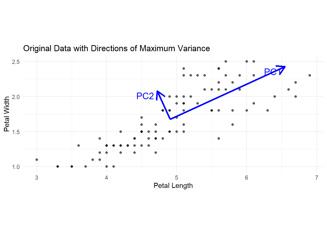
Principal components are the key to understanding the correlations between variables. They are vectors that point in the directions of the most variance. The first principal component accounts for the largest possible variance, the second PC accounts for the second largest possible variance, and so on. In Figure 1 we can see that, for two species of irises, the most variance is along the “best fit” line, and the second most variance is along the line orthogonal (perpendicular) to the first. These principal components are the eigenvectors of the data sets.
Principal components will always be orthogonal to each other since they have to catch “new variance” that is not explained by the direction of any other principal component. In two and three dimensions this is pretty easy to visualize, but it gets harder with adding variables.
You can also see that the principal components are not the same size. These eigenvectors are scaled by a value that describes “how much” variance is observed. This factor is the eigenvalue (\(\lambda\)) of the corresponding eigenvector. Note: In Figure 1, the eigenvalues are scaled by square roots for visibility. We will review how to find eigenvalues and eigenvectors in the following section.
Code
library(ggplot2)library(ggrepel)library(dplyr)# Use petal length and width from irisdata <- iris |>filter(Species !="setosa") |>select(Petal.Length, Petal.Width)# Calculate the meandata_mean <-colMeans(data)# Center the data (for correct PCA calculation)centered_data <-scale(data, center =TRUE, scale =FALSE)# Compute covariance matrixcov_matrix <-cov(centered_data)# Eigen decompositioneig <-eigen(cov_matrix)# Eigenvectors and eigenvalueseig_vectors <- eig$vectorseig_values <- eig$valuesorder_index <-order(eig$values, decreasing =FALSE)eig_vectors <--eig$vectors[, order_index]eig_values <- eig$values[order_index]# Create a data frame for eigenvectors (scaled by sqrt of eigenvalues for visibility)arrows_df <-as.data.frame(eig_vectors)arrows_df$PC <-c("PC2", "PC1")arrows_df$length <-sqrt(eig_values) # scale by variance explainedarrows_df$xend <- data_mean[1] + arrows_df$V1 * arrows_df$length *2arrows_df$yend <- data_mean[2] + arrows_df$V2 * arrows_df$length *2arrows_df$x <- data_mean[1]arrows_df$y <- data_mean[2]# Plot the original dataggplot(data, aes(x = Petal.Length, y = Petal.Width)) +geom_point(alpha =0.6) +geom_segment(data = arrows_df,aes(x = x, y = y, xend = xend, yend = yend),arrow =arrow(length =unit(0.2, "inches")),color ="blue", size =1.2) +geom_text_repel(data = arrows_df,aes(x = xend, y = yend, label = PC),color ="blue", size =5) +labs(title ="Original Data with Directions of Maximum Variance",x ="Petal Length",y ="Petal Width") +coord_fixed() +# Keep 1:1 aspect ratio so directions aren't distortedtheme_minimal()
Figure 1
The Steps to Performing Principal Component Analysis
Now that we have set the foundation, it’s time to go over the steps to performing a principal component Analysis.
1. Standardize the Given Data
This first step is a common statistics one, and it is necessary in preparing the data. Say you are comparing, in inches, human height to fingernail length. The ranges for those attributes are wildly different, and with how principal components are found, the larger range would be perceived as “more varied” and thus dominate.
This can be avoided by standardizing the data by comparing the points relative to their sample means and standard deviations. If you’ve ever taken a statistics course, this equation will be familiar: \[
z = \frac{x - \bar{x}}{\sigma}
\]
\(x\) is the variable value
\(\bar{x}\) is the sample mean for that variable
\(\sigma\) is the sample standard deviation
\(z\) is the resulting standardized value
Sample mean and sample standard deviation can both be calculated, but standard deviation in particular can be lengthy to do by hand. Applying this formula for each variable will create a new plot with coordinates centered around the origin.
2. Compute the Covariance Matrix
A covariance matrix is simply an \(n \times n\) matrix that contains the covariances between \(n\) variables “Covariance Matrix” (2025). The covariance matrix describes how variables vary from the mean with respect to each other. An example for three variables \(x\), \(y\), and \(z\) is shown below: \[
Cov(x,y,z) = \left[ \begin{array}{ccc} Cov(x,x) & Cov(x,y) & Cov(x,z) \\ Cov(y, x) & Cov(y,y) & Cov(y,z) \\ Cov(z,x) & Cov(z,y) & Cov(z,z) \end{array} \right]
\] The covariance matrix is defined as follows: \[ M = \frac{1}{n-1}X^TX \] Where \(X\) is the mean-subtracted data, and \(X^T\) is the transpose of that matrix. Explaining how covariance is calculated will reveal some more insights about why the matrix is defined in this way.
Computing variance and covariance
Sample variance is defined as \[
Var(x) = \sigma^2 = \frac{\sum_{i = 1}^{n} (x_i-\bar{x})^2}{n-1}
\]
\(X_i\) indicates the “\(i\)th” observation
\(\bar{x}\) is the sample mean
\(n\) is the number of observations
\(\sigma\) we already saw is standard deviation, so variance is just \(\sigma^2\) (now you can see why calculating standard deviation by hand is burdensome)
Sample covariance is defined similarly:
\[ Cov(x,y) = \frac{\sum_{i = 1}^{n} (x_i-\bar{x})(y_i-\bar{y})}{n-1} \] Now that we know the calculations for variance and covariance, the definition for a covariance matrix makes sense. Here’s a quick three-entry example in \(\mathbb{R}^2\):
Realize that covariance is commutative and thus \(M = M^T\). Each entry is just the sum of mean-reduced products and, once divided by \(n-1\), matches the formula for covariance shown earlier.
Notice that \(Cov(x,x)\) is the same as \(Var(x)\) and likewise for the other covariances along the diagonal. Due to the commutative properties mentioned earlier, the values on either side of the diagonal are the same. From this, we realize that the covariance matrix is symmetric.
Why a symmetric matrix is important
As a consequence of the Spectral Theorem any real symmetric matrix has a full set of real eigenvalues and orthogonal eigenvectors Knill (n.d.). This is crucial since, as already mentioned, orthogonality avoids doubly accounting for variance already described by one eigenvector. For the \(2\times 2\) matrix example performed earlier, there will be two real eigenvalues corresponding to two orthogonal eigenvectors.
3. Compute Eigenvalues and Eigenvectors
We’ve talked at length about the importance of eigenvalues and eigenvectors, but now we actually get into computing them.
As a refresher, an eigenvalue of a square matrix \(A\) is a scalar \(\lambda\) such that for a non zero vector \(\mathbf{v}\), \(A\mathbf{v} = \lambda\mathbf{v}\). As mentioned in the introduction, we can think of \(\lambda\) as a scaling factor for the principal components (eigenvectors). Since variances are always positive (\(\sigma^2\)), the eigenvalues will be too; it’s only a matter of magnitude (\(\lambda = 0\) indicates no correlation).
Since we know that the covariance matrix will have \(n\) eigenvalues, we can use \(\det(A-\lambda I) = 0\) to solve for the eigenvalues. Rearranging the original equation, we get \(A\mathbf{v} = \lambda\mathbf{v} \rightarrow a\mathbf{v} - \lambda\mathbf{v} = 0 \rightarrow (A-\lambda)\mathbf{v} = 0\). Solving for \(\mathbf{v}\) we get the eigenvectors associated with the eigenvalues. We will go into more detail about computing eigenvalues and eigenvectors in the full example walkthrough.
4. Determine the Dominant Eigenvectors
To determine which eigenvectors to hold onto (and eventually project onto), we must look at the prominence of their corresponding eigenvalues. This can be done by finding the percent influence of each eigenvalue. For example, if \(\lambda_1 = 0.95\) and \(\lambda_2 = 0.05\), then \(\lambda_1\) accounts for 95% of the variance in the sample. Discarding \(\lambda_2\) will result in a 5% loss of information but simplifies the analysis. Note: eigenvalues will not necessarily sum to 1. Values in this example were chosen for convenience.
5. Project Coordinates along Eigenvector Axes
In this final step, we project the coordinates onto the subspace whose axes are the remaining principal components.
Projection generally
Projecting one vector onto another is common practice in not just linear algebra but also vector calculus. The formula is described by
\[ proj_\mathbf{u}\mathbf{v} = \frac{(\mathbf{v}\cdot\mathbf{u})\mathbf{u}}{\mathbf{u}\cdot\mathbf{u}} \] where \(\mathbf{u}\) is the vector we’re projecting onto (the remaining eigenvectors in the case of PCA) and \(\mathbf{v}\) is the vector we are projecting.
There is error involved with this since the distance between the two vectors is being “collapsed” as one is projected onto the other. Using basic vector algebra we can describe that error with the equation \(\mathbf{e} = \mathbf{y} - \hat{y}\) where \(\mathbf{y}\) is the vector being projected onto \(\hat{y}\). This is important to consider knowing that information loss is inevitable during PCA.
Projecting onto subspaces with orthogonal vectors
We can take advantage of the fact that the eigenvectors are orthogonal, so we don’t have to worry about overlap when we take dot products. Additionally, if we normalize the eigenvectors, so their magnitudes are 1, then we don’t have to worry about scaling.
To normalize a vector, divide the components by the vector’s magnitude (\(\frac{\mathbf{v}}{||\mathbf{v}||}\)).
Since we’re usually projecting points onto a subspace, like \(\mathbb{R}^2\), we will have a matrix \(U_k\) whose columns are the top \(k\) Principal Components of interest. This matrix is left multiplied by the matrix \(X\) which contains all the centered data points. During this process we are essentially taking the dot product of each eigenvector with each coordinate. Below is an example of taking three, three-dimensional entries and reducing them to \(\mathbb{R}^2\).
We have the same number of points as before, but now they exist in \(\mathbb{R}^2\) instead of \(\mathbb{R}^3\).
A conceptual note
After performing PCA, the transformed coordinate space is typically not aligned with the original variables unless those variables are completely uncorrelated. For example, if we begin with the variables “height” and “weight”, PCA might reduce the data to a single principal component — a new axis that doesn’t represent height or weight alone, but a linear combination of the two. We might interpret this axis as representing the general notion of “size”, where points farther along the positive direction of the component indicate individuals who are overall larger. As the relationship between height and weight changes — say, becoming more heavily influenced by height — the interpretation of the principal component may shift. We can either decide that “size” is not a good descriptor of the principal component, or we can change our perspective on what “size” actually represents.
Understanding this basic example is useful when considering higher dimensional spaces created by principal components. We must consider the relative influences of principal components to form a conceptual understanding of what the trends in the data are truly suggesting.
Full Example Problem Walkthrough
Let’s work through performing PCA on a small data set. Say we’re given this table with information about five athletes:
Code
# Load knitrlibrary(knitr)# Create the data frameathletes <-data.frame(Athlete =c("Athlete 1", "Athlete 2", "Athlete 3", "Athlete 4", "Athlete 5"),Height_cm =c(180, 175, 190, 185, 178),Weight_kg =c(75, 68, 85, 80, 72),Arm_Span_cm =c(182, 176, 193, 188, 180))# Display as a kablekable(athletes, caption ="Measurements of 5 Athletes")
Table 1: Measurements of 5 Athletes
Athlete
Height_cm
Weight_kg
Arm_Span_cm
Athlete 1
180
75
182
Athlete 2
175
68
176
Athlete 3
190
85
193
Athlete 4
185
80
188
Athlete 5
178
72
180
We can convert these values into a \(5 \times 3\) matrix.
Using the formula \(\bar{x} = \frac{\sum_{i = 1}^{N} x_i}{N}\) for averages and \(\sigma = \sqrt\frac{\sum_{i = 1}^{N}(x_i-\bar{x})^2}{N-1}\) for standard deviation, we find:
\[ \mathbf{v}_1 = \left[ \begin{array}{c} 1.0123 \\ 1.0228 \\ 1 \end{array} \right]\] Performing the same operations but substituting in \(\lambda_2\) and \(\lambda_3\) we get:
These three vectors point in the directions of most variance. Recognize that \(\lambda_1\) is much larger than \(\lambda_2\) or \(\lambda_3\), so \(\mathbf{v}_1\) will explain almost all the variance (~99%). We will thus select \(\mathbf{v}_1\) to project our original, standardized points onto. To avoid needing to scale the dot product later, we can normalize \(\mathbf{v}_1\).
\[\mathbf{v}_n = \frac{\mathbf{v_1}}{||\mathbf{v_1}||} = \frac{1}{\sqrt{1.0123^2+1.0228^2+1}}\left[ \begin{array}{c} 1.0123 \\ 1.0228 \\ 1 \end{array} \right] = \left[\begin{array}{c}0.577 \\ 0.583 \\ 0.570\end{array}\right]\] We can finally take the dot product of each row of our standardized data \(Z\) with \(\mathbf{v}_n\) to get a list of values corresponding to athletes 1 through 5.
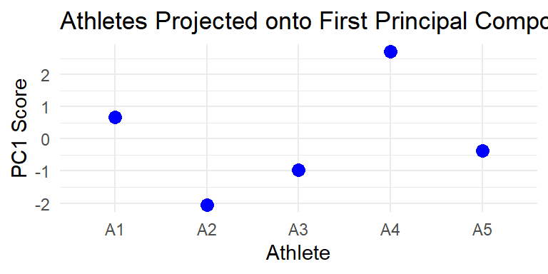
\[ Z_{reduced} = Z\mathbf{v}_n = \left[ \begin{array}{ccc}0.43 & 0.23 & 0.50 \\ -1.19 & -1.19 & -1.17 \\ -0.65 & -0.48 & -0.54 \\ 1.51 & 1.64 & 1.54 \\ -0.11 & -0.20 & -0.33 \end{array} \right]\left[\begin{array}{c}0.577 \\ 0.583 \\ 0.570\end{array}\right] = \left[\begin{array}{c}0.667\\-2.048\\-0.963\\2.706\\-0.368\end{array}\right]\] We can call the correlation between height, weight, and arm span “size” and imagine putting these values on a dot plot like in Figure 2 where more positive numbers indicate a “bigger” individual than smaller numbers. Using this definition, Athlete 4 is the “biggest” and Athlete 2 is the “smallest” of this group. Adding more athletes may shift the center and/or variance, adjusting our interpretation.
Code
library(ggplot2)# Create the data frame with the PC1 values for each athletedf <-data.frame(Athlete =factor(c("A1", "A2", "A3", "A4", "A5"), levels =c("A1", "A2", "A3", "A4", "A5")),PC1 =c(0.667, -2.048, -0.963, 2.706, -0.368))# Create a dot plot with athletes on x-axisggplot(df, aes(x = Athlete, y = PC1)) +geom_point(color ="blue", size =3) +labs(title ="Athletes Projected onto First Principal Component",x ="Athlete",y ="PC1 Score") +theme_minimal()
Figure 2
Singular Value Decomposition
Singular Value Decomposition (SVD) is a method of matrix factorization that simplifies analysis by breaking an \(m\times n\) matrix \(X\) into three simple matrices “Singular Value Decomposition(Svd)” (2021):
\[ X = U\Sigma V^T\]
\(U\): \(m\times n\) orthogonal matrix of left singular vectors
\(\Sigma\): \(m\times n\) diagonal matrix of singular values
\(V^T\): transpose of \(n\times n\) orthogonal matrix of right singular vectors
Since \(X\) can be any real \(m\times n\) matrix, we left multiply it by its transpose \(X^T\) to give us a square, \(n\times n\) matrix that will be easier to work with. The newly created \(X^TX\) captures the correlation between columns of \(X\). Remembering the covariance matrix from earlier, we recall that the diagonal was simply the variances \(\sigma^2\) of each variable. Singular values (\(\sigma\)) are the square root of the eigenvalues of the matrix \(X^TX\). Singular values tell us how much of a data set’s variance lies in the corresponding direction.
The right singular vectors (\(\mathbf{v}\)) are just the vectors found by solving \((X^TX - \sigma^2)\mathbf{v} = 0\). \(\sigma^2\) takes the place of where \(\lambda\) originally was. The left singular vectors (\(\mathbf{u}\)) are found by projecting the matrix \(X\) onto the right singular vectors (\(\mathbf{u} = X\mathbf{v}\)).
Relevance to PCA
SVD can be used to perform PCA after the data set is standardized. The columns of \(V\) are just the principal components (eigenvectors) that we would have otherwise needed to compute from the covariance matrix. The eigenvalues of the covariance matrix are the squares of the singular values. Singular values determine the amount of variance in a direction, and squaring these values will give explained variance – the objective of PCA.
SVD allows us to work directly with standardized data and skip constructing a covariance matrix which would be an intensive process if our data set is large (unlike our walkthrough example).